All JEE Main Maths Formulas
Every formula across all chapters in one place. Jump to any chapter or scroll through the complete collection.
 New
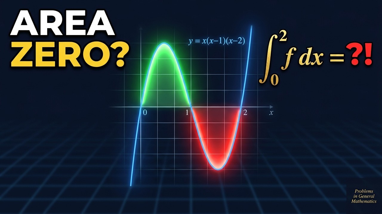
NewThe integral that lies. Why this area is not zero.
This definite integral looks perfectly symmetric, so most students write zero on sight. It is not zero, and the video shows exactly why that quick symmetry argument quietly breaks down here.
Complex Numbers & Quadratic Equations
12 formulasModulus of a Complex Number
#1💡 Always non-negative. |z| = 0 iff z = 0.
Argument of z
#2💡 Check the quadrant! tan⁻¹ alone gives values in (-π/2, π/2).
Polar Form
#3💡 r = |z|, θ = arg(z). Euler's form is faster for multiplication.
Conjugate Properties
#4💡 z·z̄ = |z|² is used everywhere - division, modulus proofs, locus.
Modulus of Product & Quotient
#5💡 Arguments add for product, subtract for quotient.
De Moivre's Theorem
#6💡 Works for all integers n. Key for finding nth roots.
nth Roots of Unity
#7💡 They form a regular n-gon on the unit circle. Sum = 0, Product = (-1)^{n+1}.
Cube Roots of Unity
#8💡 ω = (-1+i√3)/2. Used heavily in factoring and symmetric expressions.
Triangle Inequality
#9💡 Equality in upper bound when arg(z₁) = arg(z₂). Lower bound when arg differ by π.
Circle in Complex Plane
#10💡 |z − a| = |z − b| is the perpendicular bisector of segment ab.
Straight Line in Complex Plane
#11💡 arg((z-a)/(z-b)) = θ gives an arc of a circle through a and b.
Quadratic with Complex Roots
#12💡 Complex roots always come in conjugate pairs for real polynomials.
Sequence & Series
10 formulasnth Term of AP
#1💡 a = first term, d = common difference. Works for any integer n.
Sum of n Terms of AP
#2💡 l = last term. Second form is faster when you know the last term.
nth Term of GP
#3💡 a = first term, r = common ratio. Valid for all positive integers n.
Sum of n Terms of GP
#4💡 Use (1-r^n)/(1-r) when |r|<1 to avoid sign confusion.
Sum of Infinite GP
#5💡 Only converges when |r|<1. This is the most tested GP formula in JEE.
Sum of First n Natural Numbers
#6💡 Building block for all summation formulas.
Sum of Squares
#7💡 Frequently appears in method-of-differences and series summation.
Sum of Cubes
#8💡 Sum of cubes = (sum of first n numbers) squared. Elegant identity.
Sum of AGP
#9💡 Multiply S by r, subtract from S to reduce the AP part. Works every time.
Method of Differences
#10💡 If first differences form an AP or GP, use this to find the general term.
Permutations & Combinations
8 formulasPermutations (nPr)
#1💡 Order matters. Number of ways to arrange r items from n distinct items.
Combinations (nCr)
#2💡 Order does not matter. Selection of r items from n distinct items.
Permutations with Repetition
#3💡 n total items with p_1 identical of type 1, p_2 of type 2, etc.
Circular Permutations
#4💡 Fix one object and arrange the rest. For necklace/bracelet, divide by 2.
Stars and Bars
#5💡 n identical items into r distinct groups (each group can be empty).
Pascal's Identity
#6💡 Basis of Pascal's triangle. Useful for recursive counting arguments.
Derangements
#7💡 Number of permutations where no element is in its original position.
Numbers Divisible by k
#8💡 Divisibility by 3/9: digit sum divisible. By 4: last 2 digits. By 8: last 3 digits.
Binomial Theorem
8 formulasBinomial Theorem
#1💡 n must be a non-negative integer. Total (n+1) terms.
General Term
#2💡 The (r+1)th term. r starts from 0. For finding a specific coefficient, set the power of x equal to the required value and solve for r.
Middle Term(s)
#3💡 Even n: one middle term. Odd n: two middle terms. The middle term often has the greatest binomial coefficient.
Sum of Binomial Coefficients
#4💡 Put x=1 in (1+x)^n. Sum of all coefficients of (1+x)^n is 2^n.
Alternating Sum
#5💡 Put x=-1 in (1+x)^n. Even-indexed and odd-indexed coefficients have equal sum.
Sum of Coefficients of f(x)
#6💡 To find sum of all coefficients in any expansion, substitute x=1. Works for any polynomial expression.
Integral/Rational Terms
#7💡 For (a^{1/p} + b^{1/q})^n, the term is rational only when both exponents are integers.
Remainder using Binomial
#8💡 Write the base as (multiple of divisor ± small number). All terms except the last are divisible.
Matrices & Determinants
10 formulasDeterminant of 2×2 Matrix
#1💡 Product of main diagonal minus product of off-diagonal.
Determinant of 3×3 Matrix
#2💡 Expand along the row/column with most zeros to simplify calculation.
Determinant of Product
#3💡 Works for square matrices of same order. Also |A^n| = |A|^n.
Adjoint and Inverse
#4💡 adj(A) = transpose of cofactor matrix. |adj(A)| = |A|^{n-1} for n×n matrix.
Scalar Multiple of Determinant
#5💡 Each of the n rows gets multiplied by k, so the determinant picks up k^n.
Cramer's Rule
#6💡 D ≠ 0: unique solution. D = 0 and all Dᵢ = 0: infinite or no solutions. D = 0 and some Dᵢ ≠ 0: no solution.
Characteristic Equation (2×2)
#7💡 tr(A) = sum of diagonal elements = sum of eigenvalues. |A| = product of eigenvalues.
Cayley-Hamilton Theorem
#8💡 For 2×2: A² - tr(A)·A + |A|·I = O. Use this to express A⁻¹ in terms of A and I.
Orthogonal Matrix
#9💡 Rotation matrices are orthogonal. If det = 1, it's a proper rotation.
Nested Adjoint
#10💡 For adj applied k times: det = |A|^{(n-1)^k}. Very common in JEE numerical problems.
Probability
8 formulasConditional Probability
#1💡 Read as 'probability of A given B'. Reduces the sample space to B.
Bayes' Theorem
#2💡 Use when you know the result and want to find which cause produced it. 'Reverse' conditional probability.
Total Probability
#3💡 E₁, E₂, ..., Eₙ must be a partition of the sample space (mutually exclusive, exhaustive).
Binomial Distribution
#4💡 n independent trials, each with success probability p. Mean = np, Variance = npq.
Mean & Variance of Binomial
#5💡 For binomial, Var(X) < E(X) since q < 1. If Var > Mean, it's NOT binomial.
Independent Events
#6💡 Independence ≠ mutually exclusive. If A and B are mutually exclusive and both have non-zero probability, they are NOT independent.
Expectation & Variance
#7💡 Var(aX+b) = a²Var(X). E(aX+b) = aE(X)+b. Variance is always non-negative.
Addition Theorem
#8💡 For mutually exclusive events: P(A ∪ B) = P(A) + P(B). Extend for 3 events using inclusion-exclusion.
Straight Lines
8 formulasSlope-Intercept Form
#1💡 m = slope, c = y-intercept. Slope = tan(θ) where θ is angle with positive x-axis.
Two-Point Form & Slope Formula
#2💡 Slope is undefined for vertical lines (x₁ = x₂).
Distance from Point to Line
#3💡 Line: ax + by + c = 0. Don't forget the absolute value. Distance between parallel lines: |c₁-c₂|/√(a²+b²).
Angle Between Two Lines
#4💡 For perpendicular lines: m₁m₂ = -1. For parallel lines: m₁ = m₂.
Family of Lines
#5💡 Passes through the intersection of L₁ = 0 and L₂ = 0 for all values of λ. Choose λ to satisfy additional conditions.
Area of Triangle (Coordinate)
#6💡 Area = 0 means the points are collinear. Can also use determinant form.
Section Formula
#7💡 Internal division: both +. External division: replace n with -n. Midpoint: m = n = 1.
Image of Point in a Line
#8💡 Line: ax + by + c = 0. The foot of perpendicular uses the same formula but with -1 instead of -2.
Definite & Indefinite Integrals
10 formulasPower Rule
#1💡 For n = -1: ∫(1/x)dx = ln|x| + C. Always add the constant of integration for indefinite integrals.
Integration by Substitution
#2💡 Choose substitution to simplify the integrand. Don't forget to convert dx to dt and change limits for definite integrals.
Integration by Parts
#3💡 ILATE rule for choosing u: Inverse trig > Log > Algebraic > Trig > Exponential.
King's Property
#4💡 Most powerful property for definite integrals. Use when f(x) + f(a+b-x) simplifies nicely.
Even/Odd Function Property
#5💡 Check parity first for symmetric limits. Saves huge computation for odd functions (integral = 0).
Periodic Function Property
#6💡 For sin²x, cos²x: period = π. For |sinx|, |cosx|: period = π.
Walli's Formula
#7💡 k = π/2 if n is even, k = 1 if n is odd. Double factorial: n!! = n(n-2)(n-4)...
Partial Fractions
#8💡 For repeated roots: A/(x-a) + B/(x-a)². For irreducible quadratic: (Ax+B)/(x²+px+q).
Definite Integral as Limit of Sum
#9💡 Replace r/n → x, 1/n → dx. Limits: r=1 gives x=0, r=n gives x=1.
Beta Function
#10💡 Useful for integrals of the form ∫₀¹ xᵃ(1-x)ᵇ dx. Γ(n) = (n-1)! for positive integers.
Trigonometric Functions
10 formulasCompound Angle Formulas (sin, cos)
#1💡 For cos, the sign flips: cos(A+B) has minus, cos(A-B) has plus.
Compound Angle Formula (tan)
#2💡 Undefined when denominator is zero, i.e., tan A tan B = 1 for A+B case.
Double Angle Formulas
#3💡 cos 2A has three equivalent forms. Pick the one that matches the unknowns in the problem.
Half Angle Formulas
#4💡 The sign of the square root depends on the quadrant of A/2, not A. Derived from cos 2A = 1 - 2sin^2A (rearrange for sin A/2) and cos 2A = 2cos^2A - 1 (rearrange for cos A/2).
Product-to-Sum Formulas
#5💡 Useful for integrating products of trig functions and simplifying series. Derived by adding/subtracting compound angle formulas.
Sum-to-Product Formulas
#6💡 For sin C - sin D, it becomes 2 cos((C+D)/2) sin((C-D)/2). For cos C - cos D, it becomes -2 sin((C+D)/2) sin((C-D)/2).
General Solutions of Trigonometric Equations
#7💡 Always express the general solution. For specific intervals, substitute integer values of n.
Sine Rule
#8💡 R is the circumradius. Use when you know an angle and its opposite side, or need to find the circumradius.
Cosine Rule
#9💡 Use when you know all three sides (SSS), or two sides and included angle (SAS).
Area of Triangle Using Trig
#10💡 Also equals abc/(4R) using the sine rule, and rs where r is the inradius and s is the semi-perimeter.
Limits, Continuity & Differentiability
10 formulasLimit of sin x / x
#1💡 Works for radians only. Also: lim(tan x / x) = 1 and lim(sin(kx) / (kx)) = 1 as x approaches 0.
Exponential Limit (1 + x)^(1/x)
#2💡 For the general form: lim [1 + f(x)]^(1/f(x)) = e when f(x) approaches 0. Use this to handle 1^infinity forms.
Limit of (e^x - 1)/x
#3💡 Useful for converting exponential limits into simpler forms. Substitute t = e^x - 1 when needed.
Limit of (a^x - 1)/x
#4💡 Here log means log base e (natural logarithm). This follows from writing a^x = e^(x log a) and using the (e^t - 1)/t limit.
Limit of (x^n - a^n)/(x - a)
#5💡 Valid for all real n. This is essentially the derivative of x^n at x = a from first principles.
L'Hopital's Rule
#6💡 Always verify the 0/0 or infinity/infinity indeterminate form before applying. May need to be applied repeatedly.
Condition for Continuity
#7💡 All three must exist and be equal: left-hand limit, right-hand limit, and the function value at the point.
Derivative from First Principles
#8💡 Also called the limit definition of derivative. Both left-hand derivative (h approaches 0 from negative side) and right-hand derivative must be equal for differentiability.
Rolle's Theorem
#9💡 All three conditions must hold: continuity on [a,b], differentiability on (a,b), and f(a) = f(b). If any fails, the theorem cannot be applied.
Lagrange's Mean Value Theorem (LMVT)
#10💡 LMVT is a generalization of Rolle's theorem (Rolle's is the special case when f(a) = f(b)). Geometrically, the tangent at c is parallel to the secant joining (a, f(a)) and (b, f(b)).
Application of Derivatives
10 formulasRate of Change
#1💡 dy/dx gives the instantaneous rate of change of y with respect to x. For related rates, use chain rule: dy/dt = (dy/dx)(dx/dt).
Equation of Tangent
#2💡 The slope of the tangent at (x1, y1) is f'(x1). If f'(x1) = 0, the tangent is horizontal: y = y1.
Equation of Normal
#3💡 Normal is perpendicular to the tangent. Its slope = -1/f'(x1). If f'(x1) = 0, the normal is vertical: x = x1.
Length of Tangent, Normal, Subtangent, Subnormal
#4💡 Length of tangent = |y1|sqrt(1 + 1/[f'(x1)]^2). Length of normal = |y1|sqrt(1 + [f'(x1)]^2). These are measured from the point to the x-axis intercept along tangent/normal.
Condition for Increasing Function
#5💡 f'(x) >= 0 (with equality only at isolated points) also gives strictly increasing. Check open interval for derivative sign.
Condition for Decreasing Function
#6💡 Similar to increasing: f'(x) <= 0 (with equality only at isolated points) also gives strictly decreasing.
First Derivative Test
#7💡 Find critical points where f'(x) = 0 or f'(x) does not exist. Check sign of f'(x) on either side of each critical point.
Second Derivative Test
#8💡 If f''(c) = 0, the test is inconclusive. Fall back to the first derivative test in that case.
Global Max/Min on Closed Interval [a, b]
#9💡 Evaluate f at all critical points inside (a, b) AND at both endpoints a and b. The largest value is the global max, smallest is the global min.
Linear Approximation
#10💡 Used to approximate values like sqrt(4.01), (3.98)^(1/2), etc. Choose x as the nearest value where f is easy to compute.
Differential Equations
10 formulasOrder and Degree of a Differential Equation
#1💡 Order is always defined. Degree is defined only when the DE is a polynomial in its derivatives. If sin(y') or e^(y'') appears, degree is not defined.
Variable Separable Form
#2💡 Separate all y terms (with dy) to one side and all x terms (with dx) to the other, then integrate both sides.
Homogeneous Differential Equation
#3💡 After solving for v, substitute back v = y/x to get the solution in terms of x and y.
Linear First-Order DE
#4💡 First rewrite the DE in standard linear form. The integrating factor (IF) multiplies both sides. Remember: the formula also works as dx/dy + P(y)x = Q(y).
Bernoulli's Equation
#5💡 After substituting v = y^(1-n), the equation reduces to a linear DE in v. Solve that linear DE, then convert back to y.
Exact Differential Equation
#6💡 Solution: integrate M w.r.t. x (treating y as constant), then add terms from N that are not already present. The solution is F(x,y) = C.
Formation of DE by Eliminating Constants
#7💡 The order of the resulting DE equals the number of arbitrary constants in the family of curves.
Orthogonal Trajectories
#8💡 Orthogonal trajectories cut the given family at right angles. After replacement, solve the new DE to get the trajectory equation.
Exponential Growth and Decay
#9💡 k > 0 for growth, k < 0 for decay. Half-life: t_{1/2} = log(2)/|k|. Use log, not ln, per JEE convention.
Newton's Law of Cooling
#10💡 T_s is the surrounding temperature, T_0 is the initial temperature of the body, and k > 0. The body cools exponentially toward T_s.
Conic Sections
10 formulasStandard Parabola y² = 4ax
#1💡 Vertex at origin. Axis along x-axis. For y² = -4ax, the parabola opens leftward. Latus rectum (LR) passes through the focus, perpendicular to the axis.
Standard Ellipse
#2💡 Here a > b. If b > a, the major axis is along the y-axis and eccentricity uses a²/b². For an ellipse, 0 < e < 1 always.
Standard Hyperbola
#3💡 For a hyperbola, e > 1 always. The conjugate hyperbola is x²/a² - y²/b² = -1. Relationship: b² = a²(e² - 1).
Tangent to Parabola in Slope Form
#4💡 This is the tangent to y² = 4ax with slope m. The point of contact is (a/m², 2a/m). For m = 0, the tangent is at infinity.
Tangent to Ellipse in Slope Form
#5💡 The condition for y = mx + c to be tangent to the ellipse is c² = a²m² + b². Two tangents exist for each slope (one on each side).
Condition for Tangency to Conics
#6💡 For parabola y² = 4ax: c = a/m. Note the sign difference between ellipse (+b²) and hyperbola (-b²).
Focal Chord Property
#7💡 For parabola y² = 4ax, the semi-latus rectum l = 2a. If PQ is a focal chord with parameters t₁ and t₂, then t₁t₂ = -1.
Director Circle
#8💡 The director circle is the locus of the point from which two perpendicular tangents are drawn. For hyperbola, it exists only when a > b.
Chord of Contact (T = 0)
#9💡 T = 0 gives chord of contact from external point (x₁, y₁). Same equation works for tangent at a point on the curve. For pair of tangents: SS₁ = T².
Parametric Forms of Conics
#10💡 Parametric form simplifies tangent and normal equations. For parabola, slope of tangent at parameter t is 1/t.
Vectors
10 formulasMagnitude of a Vector
#1💡 Also called the modulus or length. Always non-negative. |a| = 0 only for the zero vector.
Dot Product
#2💡 Result is a scalar. theta is the angle between the two vectors. Dot product is commutative: a.b = b.a.
Cross Product Magnitude
#3💡 Result is a vector perpendicular to both a and b (right-hand rule). Cross product is NOT commutative: a x b = -(b x a).
Scalar Triple Product
#4💡 Result is a scalar. Cyclic permutation does not change the value: [a b c] = [b c a] = [c a b]. Swapping two vectors changes the sign.
Projection of a on b
#5💡 This gives a scalar (the component of a along b). For the vector projection, multiply by the unit vector of b.
Area of Triangle
#6💡 Here a and b are vectors representing two sides of the triangle from a common vertex.
Area of Parallelogram
#7💡 Parallelogram area is exactly twice the triangle area formed by the same two vectors.
Volume of Parallelepiped
#8💡 Take the absolute value of the scalar triple product. Volume is always non-negative.
Condition for Coplanarity
#9💡 Three vectors are coplanar if and only if their scalar triple product is zero. Equivalently, the 3x3 determinant of their components is zero.
Section Formula
#10💡 Divides the line segment from A (position vector a) to B (position vector b) in the ratio m:n internally. For external division, use m:(-n).
3D Geometry
10 formulasDirection Cosine Relation
#1💡 Direction cosines (l, m, n) are the cosines of the angles a line makes with the positive x, y, z axes. They always satisfy l^2 + m^2 + n^2 = 1.
Symmetric Form of a Line
#2💡 Here (x1, y1, z1) is a point on the line and (a, b, c) are direction ratios of the line. If any DR is zero, the corresponding numerator must also be zero.
General Equation of a Plane
#3💡 Here (a, b, c) are the direction ratios of the normal to the plane. The normal vector is n = a i + b j + c k.
Angle Between Two Lines
#4💡 Use direction ratios (a1, b1, c1) and (a2, b2, c2) of the two lines. Take the absolute value of the numerator to get the acute angle.
Angle Between a Line and a Plane
#5💡 theta is measured between the line and the plane (not the normal). The formula uses sin, not cos. Here (l, m, n) are DRs of the line and (a, b, c) are DRs of the normal to the plane.
Distance from a Point to a Plane
#6💡 Substitute the point (x1, y1, z1) directly into ax + by + cz + d. The absolute value ensures a non-negative distance.
Shortest Distance Between Skew Lines
#7💡 Lines: r = a1 + t*b1 and r = a2 + s*b2. Compute b1 x b2 first, then dot it with (a2 - a1). Take the absolute value and divide by |b1 x b2|.
Condition for Coplanarity of Two Lines
#8💡 Two lines are coplanar (intersect or are parallel) if and only if the shortest distance between them is zero. This is equivalent to the scalar triple product being zero.
Foot of Perpendicular from Point to Plane
#9💡 The foot lies on the line through (x1, y1, z1) with DRs (a, b, c) (the normal direction). Substitute the parametric point into the plane equation to find the parameter value.
Image of a Point in a Plane
#10💡 The image is obtained by going twice the distance from the point to the plane along the normal. The parameter value is exactly double that of the foot of perpendicular.
Circles
10 formulasGeneral Equation of a Circle
#1💡 Center is (-g, -f) and radius is sqrt(g^2 + f^2 - c). The radius is real only when g^2 + f^2 - c > 0.
Standard Form of a Circle
#2💡 Center is (h, k) and radius is r. This is the most direct form when center and radius are known.
Tangent from an External Point
#3💡 For the circle x^2 + y^2 = a^2, the tangent y = mx + c requires c^2 = a^2(1 + m^2). From an external point, there are exactly two tangents.
Length of Tangent from External Point
#4💡 S1 is obtained by substituting the external point (x1, y1) into the circle equation. This works only when the point is outside the circle (S1 > 0).
Chord of Contact T = 0
#5💡 The chord of contact from an external point (x1, y1) to the circle is obtained by replacing x^2 with xx1, y^2 with yy1, x with (x+x1)/2, and y with (y+y1)/2.
Power of a Point
#6💡 Power is positive if the point is outside, zero if on the circle, and negative if inside. It equals (distance from center)^2 - r^2.
Radical Axis of Two Circles
#7💡 The radical axis is the locus of points having equal power with respect to both circles. It is always perpendicular to the line joining the centers.
Condition for Orthogonal Circles
#8💡 Two circles are orthogonal when their tangents at the intersection points are perpendicular. This condition comes from the Pythagorean theorem applied to the triangle formed by the two centers and a point of intersection.
Parametric Form of a Circle
#9💡 Any point on the circle (x-h)^2 + (y-k)^2 = r^2 can be written as (h + r cos(theta), k + r sin(theta)). Useful for finding points on the circle satisfying additional conditions.
Director Circle
#10💡 The director circle of x^2 + y^2 = a^2 is the locus of the point from which two perpendicular tangents can be drawn to the circle. Its radius is a*sqrt(2).
Inverse Trigonometric Functions
10 formulasPrincipal Value Ranges
#1💡 Domain of sin inverse and cos inverse is [-1, 1]. Domain of tan inverse is all real numbers. The principal value is the unique value in the specified range. cosec inverse, sec inverse, and cot inverse follow from these.
Complementary Pair Identity
#2💡 Valid for all x in the respective domains. These are the most frequently used identities in JEE. They allow you to convert between inverse trig functions quickly.
Sum of Two tan inverse Values
#3💡 The condition xy < 1 vs xy > 1 determines whether the sum stays in (-pi/2, pi/2) or shifts by pi. This is the most tested formula in inverse trig.
Double Angle: 2 tan inverse x
#4💡 These identities connect tan inverse to sin inverse and cos inverse via double-angle substitution. The domain restrictions are critical and are the main source of errors.
sin inverse of 2x sqrt(1 - x^2)
#5💡 This comes from substituting x = sin(theta). The split at 1/sqrt(2) corresponds to theta = pi/4. JEE often tests this with x = sqrt(3)/2 or x = 1/sqrt(2).
Composition: sin(cos inverse x)
#6💡 Draw a right triangle with the known side to find the other trig ratio. If cos inverse(x) = theta, then cos(theta) = x, so sin(theta) = sqrt(1 - x^2).
Domain Restrictions
#7💡 cosec inverse and sec inverse have domains |x| >= 1 (excludes the interval (-1, 1)). cot inverse has domain all real numbers. These domain checks are often the first step in solving problems.
Derivative of Inverse Trig Functions
#8💡 The derivative of cos inverse is the negative of sin inverse's derivative. Similarly, cot inverse's derivative is the negative of tan inverse's. These are essential for integration as well.
tan inverse Difference Formula
#9💡 This is the difference version of the sum formula. The condition xy > -1 ensures the result is in (-pi/2, pi/2). Used heavily in telescoping series problems.
Telescoping tan inverse Series
#10💡 The key trick: 1/(1 + r + r^2) = ((r+1) - r)/(1 + r(r+1)). This makes each term a difference of two tan inverse values, leading to telescoping cancellation.
Sets, Relations & Functions
10 formulasUnion of Two Sets (Inclusion-Exclusion)
#1💡 For three sets: n(A union B union C) = n(A) + n(B) + n(C) - n(A cap B) - n(B cap C) - n(A cap C) + n(A cap B cap C). Always subtract the pairwise overlaps and add back the triple overlap.
De Morgan's Laws
#2💡 Complement of union is intersection of complements. Complement of intersection is union of complements. These hold for any number of sets.
Reflexive, Symmetric, Transitive Conditions
#3💡 Reflexive requires every element to be related to itself. Symmetric requires the relation to work both ways. Transitive requires chains to close. Check each condition independently.
Equivalence Class
#4💡 The equivalence class of a is the set of all elements related to a. Equivalence classes partition the set into disjoint, exhaustive subsets. Two elements have the same equivalence class if and only if they are related.
One-One (Injective) and Onto (Surjective) Definitions
#5💡 One-one means no two distinct inputs give the same output. Onto means every element of the codomain is hit. A function that is both one-one and onto is called bijective.
Domain of Composite Function
#6💡 For g(f(x)) to exist, x must be in the domain of f AND f(x) must be in the domain of g. Always check both conditions.
Inverse Function Existence
#7💡 Only bijective functions have inverses. If f is one-one but not onto, restrict the codomain to the range to make it bijective. If f is onto but not one-one, no inverse exists.
Number of Relations on a Set
#8💡 A relation from A to B is any subset of A x B. Since A x B has n(A)*n(B) elements, the number of subsets is 2^(n(A)*n(B)). For a relation on set A (from A to A), this becomes 2^(n(A)^2).
Number of Onto Functions (Surjections)
#9💡 Here m = n(A) and n = n(B) with m >= n. This uses inclusion-exclusion. For n(B) = 2: onto functions = 2^m - 2. For n(B) = 3: onto functions = 3^m - 3*2^m + 3.
Floor and Ceiling Functions
#10💡 Also called the greatest integer function [x]. For negative numbers: floor(-2.3) = -3, not -2. The fractional part {x} = x - floor(x) always satisfies 0 <= {x} < 1.
Statistics
10 formulasArithmetic Mean (Direct Method)
#1💡 For frequency distribution, multiply each observation by its frequency. Always check if grouped or ungrouped.
Weighted Mean
#2💡 Used when different observations carry different importance (weights). Reduces to arithmetic mean when all weights are equal.
Median (Grouped Data)
#3💡 l = lower limit of median class, N = total frequency, F = cumulative frequency before median class, f = frequency of median class, h = class width.
Mode (Grouped Data)
#4💡 f₁ = frequency of modal class, f₀ = frequency of class before modal class, f₂ = frequency of class after modal class.
Variance
#5💡 The second form (shortcut) avoids computing deviations. Var = E(X²) - [E(X)]². Always non-negative.
Standard Deviation
#6💡 SD is in the same units as the data. Variance is in squared units. SD = sqrt(Variance).
Combined Mean
#7💡 Weighted by group sizes. Extends to k groups: numerator = sum of (nᵢ times mean of group i).
Combined Variance
#8💡 where d₁ = x̄₁ - x̄₁₂ and d₂ = x̄₂ - x̄₁₂. The dᵢ terms account for the difference between group means and combined mean.
Effect of Change of Origin and Scale
#9💡 Mean changes with both origin and scale. SD changes only with scale (not origin). Variance changes by h².
Mean Deviation
#10💡 Mean deviation about the mean. Can also compute about the median. Mean deviation about the median is always minimum.
Mathematical Reasoning
10 formulasNegation of a Statement
#1💡 Negation flips the truth value. If p is 'x > 5', then ~p is 'x is not greater than 5' (i.e., x <= 5).
Conjunction (AND)
#2💡 AND requires both parts to be true. Even one false component makes the entire conjunction false.
Disjunction (OR)
#3💡 OR is inclusive in logic. It is true when at least one component is true.
Conditional (If-Then)
#4💡 A conditional is false ONLY when p is true and q is false. 'If it rains, the ground is wet' is false only when it rains but the ground is dry.
Contrapositive
#5💡 The contrapositive always has the same truth value as the original conditional. Converse (q -> p) and inverse (~p -> ~q) do NOT.
Biconditional (If and Only If)
#6💡 Biconditional is true when both p and q have the same truth value (both true or both false).
De Morgan's Laws for Logic
#7💡 Negation of AND becomes OR (with negated parts). Negation of OR becomes AND (with negated parts). Swap the connective and negate each component.
Negation of Quantifiers
#8💡 Negation of 'for all' becomes 'there exists ... not'. Negation of 'there exists' becomes 'for all ... not'. Swap the quantifier and negate the predicate.
Principle of Mathematical Induction
#9💡 Two steps: (1) Base case: verify P(1). (2) Inductive step: assume P(k) and prove P(k+1). Both steps are mandatory.
Strong Induction
#10💡 In strong induction, assume P(m) is true for ALL m from 1 to k, then prove P(k+1). Useful when P(k+1) depends on multiple previous cases, not just P(k).
Heights & Distances
10 formulasBasic Height from Angle of Elevation
#1💡 Here h is the height of the object above the observer's eye level, d is the horizontal distance, and alpha is the angle of elevation.
Angle of Elevation Definition
#2💡 The angle of elevation is always measured from the horizontal line at the observer's eye level upward to the object. It is never negative.
Angle of Depression Definition
#3💡 The angle of depression from point A to point B equals the angle of elevation from B to A (alternate interior angles). This duality is tested frequently.
Height from Two Observation Points
#4💡 Two points at distance d apart observe the top of a tower at angles alpha and beta (beta > alpha). Both observers are on the same side and at the same level as the base.
Distance Between Two Points Using Two Angles
#5💡 If a tower of height h is observed from two points on the same side, the distance between them is h(cot(alpha) - cot(beta)) where alpha < beta.
Shadow Length Formula
#6💡 Here theta is the angle of elevation of the sun. As the sun rises (theta increases), the shadow gets shorter. At theta = 45 degrees, shadow length equals height.
Sine Rule in Heights and Distances
#7💡 When the triangle formed is not right-angled (e.g., objects on hills), use the sine rule to find unknown sides or angles.
Height from Moving Observer
#8💡 Same formula as two-point observation. When a person walks d metres toward a tower and the angle changes from alpha to beta, this gives the height.
Combined Elevation and Depression
#9💡 When standing between two objects (or at the top of a building looking up at one and down at another), the total height combines both components.
Height of Object on a Hill
#10💡 When an object of height h stands on a hill inclined at angle beta, and the object subtends angle alpha at a point at the base, use this to find h.